

Data Cardinality
Visualizing Job Creation by Voting Districts in North Carolina
Problem and Objective
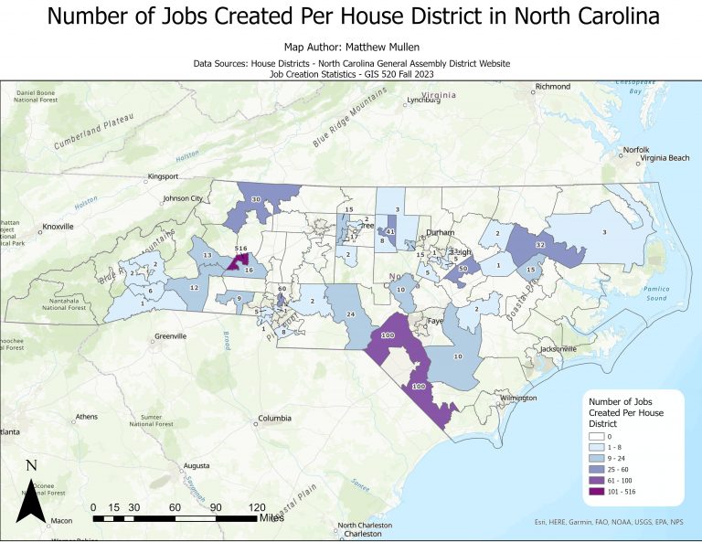
The goal of this project is to visualize job creation statistics by Senate and House districts in North Carolina. Two maps were created to display this information, job creation for each Senate district in North Carolina and one for job creation in each House district in NC. The results of this project will be valuable for NC House members and State senators to easily visualize how many jobs were created per district.
Analysis Procedures
An Excel file containing the results of an industrial extension jobs survey was provided which contains information on the number of jobs created per company and the zip code in which those jobs are worked. USA Zip Codes point data was downloaded from the ESRI website, and NC Senate and House districts from the 2018 election were obtained from the North Carolina General Assembly website. ArcGIS Pro was used for the analysis and mapping of the data. To perform the analysis needed to match job creation by zip code to Senate and House districts, Attribute Joins and Spatial Joins were used.
First, I opened the jobs survey Excel file and reviewed the data. I then summarized the data based on the total number of jobs created by company, the EMPLOY_SUM field, aggregated by zip code. This produced a file showing the total number of jobs created in each zip code. I then added the House Districts shapefile and the Senate Districts shapefile to the map, both of which used the NAD 1983 StatePlane North Carolina FIPS 3200 (Meters) projection.
From the USA Zip Codes point data, I selected only the zip codes in North Carolina. I then performed an Attribute Join of the jobs created by zip code data and the NC Zip Codes point data, using the zip code as the common field. I then selected the zip codes that had at least one job created from the newly joined data using Select by Attribute since we were only interested in job creation data. Two separate Spatial Joins were then performed that matched the zip code points with the job creation data to the House and Senate districts polygons they resided in. When setting up the Spatial Join, the attributes were summarized based on the jobs created field.
The results could then be visualized using labels showing total number of jobs created in each district and Graduated Colors symbology so the results could be understood quickly.

Results

Application & Reflection
Attribute Joins and Spatial Joins are both extremely useful analysis tools in geoprocessing. They allow data from separate tables to be combined based on a common field or location, an essential process of any geoprocessing task.
Problem description
A biologist is trying to determine if there is a link between reduced piping plover nest productivity and recorded rule violations (such as footprints inside sectioned off areas or dogs off leash in restricted areas) that occurred near the nest.
Data needed
Point data showing locations of piping plover nests and point data of rule violations recorded would be needed for this analysis, as well as data on productivity for each nest.
Analysis procedures
First the nest location data and rule violation data could be mapped. Then, an attribute join could be performed to link the nest location data with the nest productivity data if they are in separate tables. Then rule violations could be summarized by type and a spatial join could be performed to link nest locations with rule violations that occurred within a specified distance. The data could then be analyzed to see if rule violations impacted nest productivity and if the number of violations led to less productive nests. Spatially joining would also help if you wanted to create a map that showed the number of violations within a specific distance near a nest.