

Spatial Pattern Analysis
Using Spatial Analysis Tools To Determine Clustering for Service Calls at Fort Worth Fire Department and for Clustering of Library Patrons at Oleander Library
Problem and Objective
There were two main problems and objectives that were analyzed for this exercise. For the first, the Fort Worth Fire Department has asked their GIS analyst to determine if the Emergency Medical Service calls they receive have a tendency to cluster, so they can determine if they need to re-station emergency care units closer to these areas. Second, the Oleander Library in Texas would like to know if their patrons tend to cluster in certain areas for event planning purposes. The objective is to use several spatial analysis tools to quantify the cluster and either prove or disprove a null hypothesis.
Analysis Procedures
To address these problems, I used ESRI’s ArcGIS Pro version 3.1 for analysis and various tools from the Spatial Analyst toolbox including Average Nearest Neighbor, High-Low Clustering (Getis-Ord General G) tool, the Multi-Distance Spatial Clustering Analysis tool, and the Spatial Autocorrelation (Global Moran’s I) tool. The data used for the analysis included the polygon area of operation for the Battalion 2 fire department, point data for EMS calls including the urgency of each call, point data for Incidents in the Battalion 2 area, a polygon layer showing the district location of Oleander Public library and point data showing each patrons location. This data was provided by our GIS 520 class and came from the “GIS Tutorial 2 – Spatial Analyst Workbook” (4th Ed.) by David W. Allen.
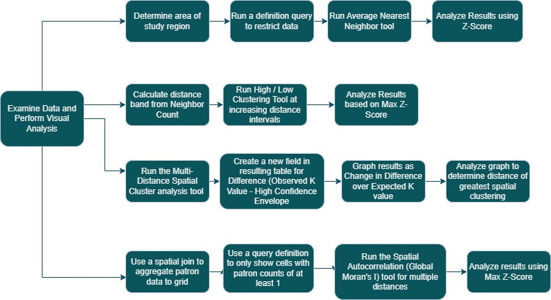
For the first three exercises, we were interested in determining if EMS calls to Fort Worth Fire Department tended to cluster in certain areas. For the first exercise, I used the Incidents layer and created a definition query to restrict the data to incidents between 700 and 740. Next, I used the Average Nearest Neighbor tool and recorded the Z-Score and confidence level reported.
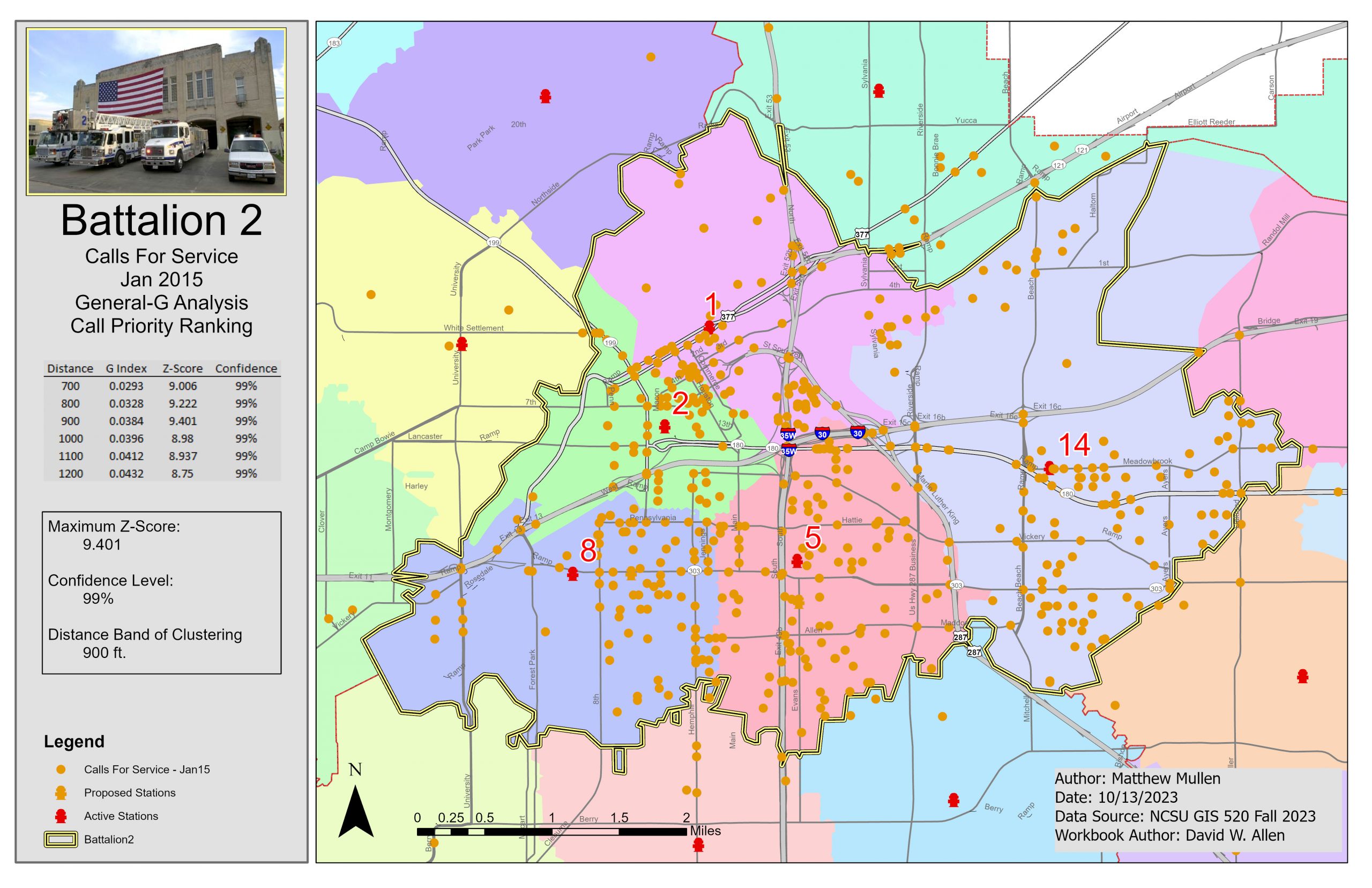
For the next exercise, I used the Calls for Service layer. I first used the Calculate Distance Band from Neighbor Count tool and determined an average neighbor distance. I then used the High/Low Clustering tool and used the FEE field (which determines the severity of the call) as the input field with the distance I determined earlier. I then reran the tool using increasing distances at an interval of 200 ft. and recorded the Z-Score, G index and confidence level of each.
For the third exercise, the Calls for Service layer was used again, and the Multi-Distance Spatial Cluster Analysis tool was utilized. The tool was run using the Battalion 2 study area, a beginning distance of 200 ft, with a distance increment of 100 feet and the weight field of call urgency (FEE). To compute the confidence envelope, 99 permutations were used. I then created a new field in the resulting table called “Difference” and populated it by subtracting the Observed K value with the High Confidence Envelope. These results were then plotted on a line graph as Change in Difference over Expected K.
For the fourth exercise, the patron data location from the Oleander Library was analyzed. First, I performed a spatial join of the 300ft. grid and the patron locations. I created a definition query to only show the cell blocks that had at least one patron. I then ran the Spatial Autocorrelation tool, starting at a distance of 2400 and incrementing by 200 ft. up to 3800 ft. The Z-Score and confidence interval was recorded for each run and I used this to make a determination of the null hypothesis. Finally, maps were created from each exercise and relevant statistics, data and conclusions were added to each map.
Results
The maps below summarize the results of the spatial pattern analysis. The nearest neighbor index produced a Z-Score of -1.698 with a confidence level of 90%, indicating there is a high probability of clustering of incident calls within the region.

The high-low clustering analysis showed the maximum clustering of calls for service occurred at the 900 ft. distance band, with a confidence level of 99%.
The multi-distance spatial cluster analysis also indicated that clustering was greatest at the 900 ft. distance band. This was determined by looking at the change in difference over the Expected K value.

This map showed that library patrons in Oleander County clustered the most at the 3400 ft. distance, with a confidence level of 99%. We were able to safely reject the null hypothesis and conclude that library patrons were clustered and not randomly dispersed within Oleander county.

Application & Reflection
The first rule of Geography states that “everything is related to everything else, but near things are more related than distant things”. Using Spatial Analyst tools we can confidently conclude whether certain events are clustered or dispersed, helping to guide our decisions. In a hypothetical scenario, I look at using Spatial Analyst tools to determine clustering of sea turtle nests on Cape Hatteras.
Problem description
I am a biologist at Cape Hatteras National Seashore and I want to determine if sea turtle nests along the seashore exhibit spatial clustering or if their nest locations are random. Additionally, I want to see if nests that have higher productivity exhibit spatial clustering to try and determine if location has a large impact on nest success.
Data needed
A point vector layer with the location of each nest found during one nesting season, along with data about each nest such as egg count, location from shore, and productivity statistics.
Analysis procedures
First, I would determine the area of the study region I am looking at. I would then use the Average Nearest Neighbor tool to calculate the distance from each feature to its nearest neighbor and record the results. I would then use the Multi-Distance Spatial Cluster Analysis tool to determine if successful nests exhibited any kind of spatial clustering. The weight field used in this analysis would be the hatch success percentage.